Código para implementação de funções de representação e manipulação de dados espaciais
vignette(package = "sf")
library(sf)
## Linking to GEOS 3.9.1, GDAL 3.2.1, PROJ 7.2.1; sf_use_s2() is TRUE
library(terra)
## terra version 1.5.2
library(spData)
## Warning: múltiplas tabelas de métodos encontradas para 'approxNA'
library(tmap)
library(tidyverse)
## -- Attaching packages --------------------------------------- tidyverse 1.3.1 --
## v ggplot2 3.3.5     v purrr   0.3.4
## v tibble  3.1.6     v dplyr   1.0.7
## v tidyr   1.1.4     v stringr 1.4.0
## v readr   2.1.1     v forcats 0.5.1
## -- Conflicts ------------------------------------------ tidyverse_conflicts() --
## x tidyr::extract()  masks terra::extract()
## x dplyr::filter()   masks stats::filter()
## x dplyr::lag()      masks stats::lag()
## x purrr::simplify() masks terra::simplify()
## x dplyr::src()      masks terra::src()
class(world)
## [1] "sf" "tbl_df" "tbl" "data.frame"
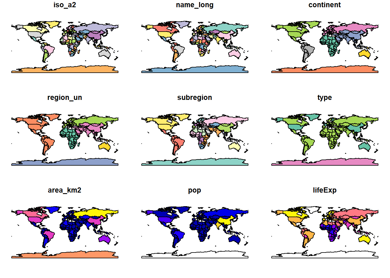
names(world)
##  [1] "iso_a2"    "name_long" "continent" "region_un" "subregion" "type"
##  [7] "area_km2"  "pop"       "lifeExp"   "gdpPercap" "geom"
plot(world)
## Warning: plotting the first 9 out of 10 attributes; use max.plot = 10 to plot
## all
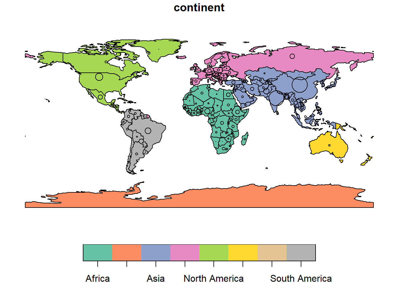
plot(world["continent"], reset = FALSE)
cex = sqrt(world$pop) / 10000
world_cents = st_centroid(world, of_largest = TRUE)
## Warning in st_centroid.sf(world, of_largest = TRUE): st_centroid assumes
## attributes are constant over geometries of x
plot(st_geometry(world_cents), add = TRUE, cex = cex)
autonomos <- st_read("shapefile/autonomos.shp")
autonomos <- st_transform(autonomos, "EPSG:4326")
st_crs(autonomos)
st_bbox(autonomos)
economica <- st_read("shapefile/economica.shp")
economica_auto <- st_transform(autonomos)
st_crs(economica_auto)
st_crs(autonomos)
new_shape <- st_transform(autonomos, "EPSG:4326") # set CRS
st_crs(new_shape)
st_bbox(autonomos)
st_bbox(new_shape)
Representação
autonomos <- st_read("shapefile/autonomos.shp")
economica <- st_read("shapefile/economica.shp")
regional <- st_read("shapefile/regional.shp")

tm_shape(regional) +
   tm_polygons("NOME",palette = "RdYlBu")

tm_shape(regional) +
   tm_borders() +
tm_shape(autonomos) +
   tm_dots(col = "red") +
   tm_scale_bar()
Manipulação de dados espaciais
farmacias <- economica %>%
   filter(CNAE_PRINC == '4771701' | CNAE_PRINC == '4771702')

tm_shape(regional) +
   tm_borders() +
tm_shape(farmacias) +
   tm_dots()
world
## Simple feature collection with 177 features and 10 fields
## Geometry type: MULTIPOLYGON
## Dimension:     XY
## Bounding box:  xmin: -180 ymin: -89.9 xmax: 180 ymax: 83.64513
## Geodetic CRS:  WGS 84
## # A tibble: 177 x 11
##    iso_a2 name_long continent region_un subregion type  area_km2     pop lifeExp
##  * <chr>  <chr>     <chr>     <chr>     <chr>     <chr>    <dbl>   <dbl>   <dbl>
##  1 FJ     Fiji      Oceania   Oceania   Melanesia Sove~   1.93e4  8.86e5    70.0
##  2 TZ     Tanzania  Africa    Africa    Eastern ~ Sove~   9.33e5  5.22e7    64.2
##  3 EH     Western ~ Africa    Africa    Northern~ Inde~   9.63e4 NA         NA
##  4 CA     Canada    North Am~ Americas  Northern~ Sove~   1.00e7  3.55e7    82.0
##  5 US     United S~ North Am~ Americas  Northern~ Coun~   9.51e6  3.19e8    78.8
##  6 KZ     Kazakhst~ Asia      Asia      Central ~ Sove~   2.73e6  1.73e7    71.6
##  7 UZ     Uzbekist~ Asia      Asia      Central ~ Sove~   4.61e5  3.08e7    71.0
##  8 PG     Papua Ne~ Oceania   Oceania   Melanesia Sove~   4.65e5  7.76e6    65.2
##  9 ID     Indonesia Asia      Asia      South-Ea~ Sove~   1.82e6  2.55e8    68.9
## 10 AR     Argentina South Am~ Americas  South Am~ Sove~   2.78e6  4.30e7    76.3
## # ... with 167 more rows, and 2 more variables: gdpPercap <dbl>,
## #   geom <MULTIPOLYGON [°]>
world_agg1 <- world %>%
group_by(continent) %>%
summarize(pop = sum(pop, na.rm = TRUE))
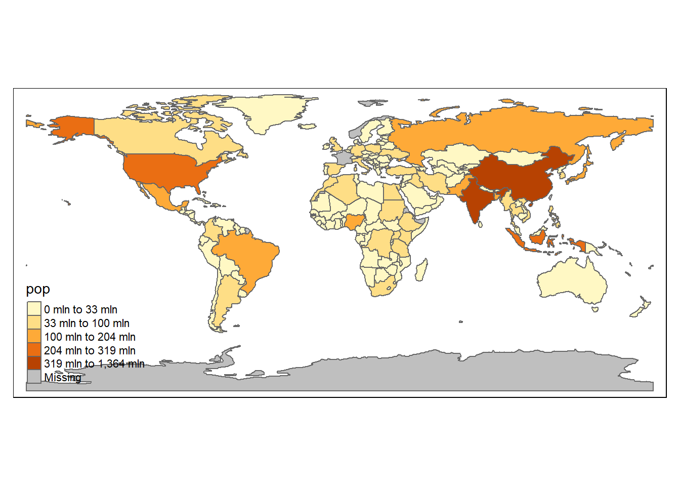
tm_shape(world) +
tm_polygons("pop", style = "jenks" )
world_agg2  <- world %>%
  group_by(continent) %>%
  summarize(pop = sum(pop, na.rm = TRUE), `area (sqkm)` = sum(area_km2), n = n())
Junção não espacial - relaciona dados por meio de uma chave
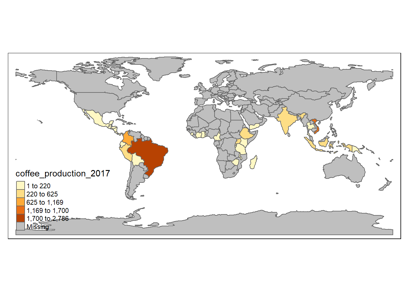
coffee_data
## # A tibble: 47 x 3
##    name_long                coffee_production_2016 coffee_production_2017
##    <chr>                                     <int>                  <int>
##  1 Angola                                       NA                     NA
##  2 Bolivia                                       3                      4
##  3 Brazil                                     3277                   2786
##  4 Burundi                                      37                     38
##  5 Cameroon                                      8                      6
##  6 Central African Republic                     NA                     NA
##  7 Congo, Dem. Rep. of                           4                     12
##  8 Colombia                                   1330                   1169
##  9 Costa Rica                                   28                     32
## 10 Côte d'Ivoire                               114                    130
## # ... with 37 more rows
juntos <- world %>%
   left_join(coffee_data)
## Joining, by = "name_long"
tm_shape(juntos) +
   tm_polygons('coffee_production_2017', style = "jenks")